2. Regression II
Introduction
Last time we looked at a simple linear regression problem in descriptive morphology and found out that it wasn’t so simple after all. In this essay I’d like to extend that analysis to consider the same problem from a slightly different angle in order to introduce another important consideration in designing such analyses, and another regression analysis method.
You will recall, our problem from the last issue was to characterise the relation between gross dimensions of the glabella for a suite of trilobite genera. Complications arose in choosing among the different ways deviations from the assumption of linearity could be calculated. Because, as is often the case with palaeontological data, no clear distinction could be drawn between glabellar length and width in terms of their dependency relations, we chose a model—the reduced major axis—that minimized the joint deviation of both variables from the model. So far so good. However, in order to determine the slope of the reduced major axis, we did something sneaky to the original length and width measurements. Something you might not have noticed, but something that changed nature of these variables utterly and would not have been needed under the least-squares regression model. We standardized them. What is standardization? Why would you want to do it? When is it appropriate? And what effect does it have on regression analyses? Those are our questions for today.
Standardization
Standardization is a procedure that allows us to compare quantitatively observations of different types. In effect, it’s a technique statisticians use for comparing apples with oranges. Palaeontologists need to make such comparisons all the time. To illustrate this let’s consider an alternative variable in which the distinction between variable types is clear. Say we wanted to determine how the length of the glabella was related to its size and had decided to use area as a measure of glabellar size. Table 1 summarizes these data for our example set of trilobite genera.
| Genus | Length (mm) | Area (mm2) |
|---|---|---|
| Acaste | 5.10 | 23.61 |
| Balizonma | 4.60 | 17.40 |
| Calymene | 12.98 | 154.22 |
| Ceraurus | 7.90 | 51.22 |
| Cheirurus | 12.83 | 158.23 |
| Cybeloides | 6.60 | 39.23 |
| Dalmanites | 10.00 | 67.40 |
| Delphion | 8.08 | 68.81 |
| Narroia | 15.67 | 127.67 |
| Ormathops | 4.53 | 14.85 |
| Phacopdina | 6.44 | 34.27 |
| Pricyclopyge | 21.53 | 250.70 |
| Ptychoparia | 12.82 | 109.40 |
| Rhenops | 22.27 | 319.56 |
| Sphaerexochus | 4.93 | 35.29 |
| Trimerus | 16.35 | 261.06 |
| Zachanthoides | 13.41 | 169.98 |
| Minimum | 4.53 | 14.85 |
| Maximum | 22.27 | 319.56 |
| Range | 17.74 | 304.71 |
| Mean | 11.25 | 120.75 |
| Variance | 32.16 | 9813.65 |
| Standard Deviation | 5.67 | 99.06 |
The summary statistics at the bottom of the table reflect what’s obvious after a moment’s reflection. Even though the measures ‘length’ and ‘area’ are closely related, they are nevertheless variables of different kinds. In the tabled values this is expressed in the gross difference between the measurement ranges. The difference between the maximum and minimum length values covers a mere 17.74 units whereas the corresponding area range value is 304.71! This difference begs the question of whether ‘length’ and ‘area’ represent the same qualities, which they clearly do not. Glabellar length is measured in mm whereas glabellar area is measured in mm2. Because of this difference, I cannot easily construct a simple, consistently scaled graph of both datasets because the scales along which the observations are arrayed are inherently different. This contrast between variable types renders direct comparisons between them difficult, even (as in this case) when the units associated with length and area exhibit a simple underlying unity.
There are a number of ways to compensate for this difference and make the two variables more directly comparable. The easiest is to transform both variables so that they exhibit a common mean value. This has the effect of centring the distributions of observations on a joint, grand mean, the most convenient value for which is zero. Table 2 shows the data presented in Table 1 after mean centring, which is accomplished by subtracting the mean value of each variable from the observed value.
| Genus | Length (mm) | Area (mm2) |
|---|---|---|
| Acaste | -6.15 | -97.14 |
| Balizoma | -6.65 | -103.35 |
| Calymene | 1.73 | 33.47 |
| Ceraurus | -3.35 | -69.53 |
| Cheirurus | 1.58 | 37.48 |
| Cybantyx | 5.16 | 149.90 |
| Cybeloides | -4.65 | -81.52 |
| Dalmanites | -1.25 | -53.35 |
| Delphion | -3.17 | -51.94 |
| Narroia | 4.42 | 6.92 |
| Ormathops | -6.72 | -105.90 |
| Phacopdina | -4.81 | -86.48 |
| Pricyclopyge | 10.28 | 129.95 |
| Ptychoparia | 1.57 | -11.35 |
| Rhenops | 11.02 | 198.81 |
| Sphaerexochus | -6.32 | -85.46 |
| Trimerus | 5.10 | 140.31 |
| Zachanthoides | 2.16 | 49.23 |
| Minimum | -6.72 | -105.90 |
| Maximum | 11.02 | 198.81 |
| Range | 17.74 | 304.71 |
| Mean | 0.00 | 0.00 |
| Variance | 32.16 | 9813.65 |
| Standard Deviation | 5.67 | 99.06 |
Note this transformation makes it much easier to compare differences in the ranges of variables about their respective means, but leaves the range of the observations unchanged. However, there’s still a problem. Because the nature of the differences between the variable types has also remained unchanged, we still can't easily portray both sets of observations on a single, consistently scaled graph. In order to achieve true comparability we need to find some other, more standard way of describing the patterns of variation present in both variables.
The solution to our problem lies in a quantity called the standard deviation. Probably most of you have heard this term. Some may know that it can be calculated by taking the square-root of the sample or population variance. But what is standard about the standard deviation?
To understand the standard deviation we need to understand the variance, which is the average1, squared deviation of all observations from the mean.
(2.1) s2=∑(xi−¯X)2/(n−1)
In this equation s2 is the standard symbol for the sample variance, xi is the ith observation or measurement, ¯X is the sample mean, and n is the sample size. The sum of the squared deviations from the sample mean is used, rather than the more intuitively obvious sum of the deviations, because the quantity ∑xi−¯X will always be 0.0 (see Table 2). Nevertheless, this sum still has a unit; and an odd unit at that. In our trilobite example, the variance of the length variable is expressed in the unit mm2 , and the variance of the area variable in the unit (mm2)2! Taking the square root of the variance returns these statistics to the units—or standard—of the original measurements.
(2.2) s=√∑(xi−¯X)2/(n−1)
Now for the trick that makes variables of fundamentally different types comparable. The significance of the standard deviation is that it tells you something about how your measurements are distributed about the mean. Because the magnitude of the standard deviation is related to the magnitude of the measurements, it’s complex to assess the meaning of a standard deviation by itself. Regardless of this magnitude though, and regardless of the shape of the distribution, the manner in which the standard deviation is calculated ensures that at least 75.00 per cent of the observations will lie within two standard deviations from the mean, and 88.89 per cent will lie within three standard deviations. If the distribution of your observations follows the normal probability density function (= a normal distribution) these percentages rise to 95.46, and 99.73 respectively. So, in principal we can get an idea of whether glabellar length has a pattern of variability greater than, equal to, or lesser than glabellar area by comparing their standard deviations. Better still, we can use the standard deviation to scale the original measurements, thereby expressing both distributions, not in terms of their non-comparable original units (mm and mm2), but in terms of a common standard-deviation scale that is comparable directly for any set of variables, irrespective of their type or the character of their distribution. This operation is termed standardization and the formula most often used to compute the standard normal form of a variable is:
(2.3) zi=xi−¯Xs
Table 3 shows the trilobite glabellar length and area data in their standardized form and Figure 1 compares the scatterplot of these raw (Table 1) and standardized data.
| Genus | Length (mm) | Area (mm2) |
|---|---|---|
| Acaste | -1.08 | -0.98 |
| Balizonma | -1.17 | -1.04 |
| Calymene | 0.31 | 0.34 |
| Ceraurus | -0.59 | -0.70 |
| Cheirurus | 0.28 | 0.38 |
| Cybeloides | 0.91 | 1.51 |
| Dalmanites | -0.82 | -0.82 |
| Delphion | -0.22 | -0.54 |
| Narroia | -0.56 | -0.52 |
| Ormathops | 0.78 | 0.07 |
| Phacopdina | -1.19 | -1.07 |
| Pricyclopyge | -0.85 | -0.87 |
| Ptychoparia | 1.81 | 1.31 |
| Rhenops | 1.94 | -0.11 |
| Sphaerexochus | -1.11 | 2.01 |
| Trimerus | 0.90 | -0.86 |
| Zachanthoides | 0.38 | 1.42 |
| Minimum | -1.19 | -1.07 |
| Maximum | 1.94 | 2.01 |
| Range | 3.13 | 3.08 |
| Mean | 0.00 | 0.00 |
| Variance | 1.00 | 1.00 |
| Standard Deviation | 1.00 | 1.00 |
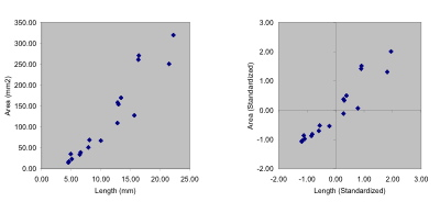
Figure 1. Scatterplots of raw (left) and standardized (right) trilobite glabellar data. Note how the standardization procedure shifts the placement and the scaling of the variables, but does not alter the positions of points relative to one another.
Where does this leave us in terms of our regression problem? As you’ll recall from last time, reduced major axis (RMA) regression calculates the regression slope as the ratio of two standard deviations. This is equivalent to performing the analysis on standardized variables. Indeed, another name for RMA regression is standard major axis regression (Jolicouer 1975). From what I’ve said above you might have the impression that it’s always best to standardize your data before analysis, in which case RMA regression would be a simple alternative to least-squares regression analysis. But recall the example we used above for exploring standardization was a comparison between glabellar lengths and areas; two very different types of variables. In our example from last time, the variables were glabellar length and width; two variables whose distributions differ in terms of their means, variances, and standard deviations, but whose units are identical. In cases like this is it appropriate to standardize the variables and then use RMA to model their linear relationship. Or, should they be left in their raw states, in which case another type of regression method will be needed?
The answer to this question is by no means straight-forward and disagreements between competent practitioners continue to surface every now and then in the technical literature. The advantage of standardization is that, through its application, non-comparable variables, or comparable variables with non-identical distributions, can be compared with the assurance that variable type and/or distributional differences are not influencing the result. The price paid for this assurance, though, is that one is no longer analyzing the variables that were measured, but a transformation of those variables in which differences in the scale and magnitude of the original observations have been, in effect, thrown away. When dealing with different types of variables this is not such a problem because it is unlikely that these qualities will be important to the comparison. After all, if one wanted to focus on issues like differences between the scale and magnitude of observations it would hardly be logical to reference those observations to variables whose scaling and magnitude are different intrinsically. In the case of variables that are measured in the same units, however, this idea of throwing away any information is troubling. Fortunately, an alternative regression method is available that allows users to minimize the joint deviation of observations from a linear model while, at the same time, preserving the flexibility to undertake their analysis on either standardized or unstandardized variables. Unfortunately, discussions of this method are even less common than those of RMA regression. The method is called major axis (or principal axis) regression analysis.
Recall that RMA regression minimized the product of the deviations from the regression line across both the and variables. This is geometrically equivalent to minimizing the area of a set of triangles in which the trace of the regression slope forms the hypotenuse (see Figure 4 from the Regression I essay). The triangle approach is a workable, but somewhat counterintuitive, minimization strategy that has the saving grace of being very simple to implement computationally, provided you are comfortable standardizing your variables. A more generalized approach would be to minimize the simple sum of the squared deviations of observed points from the model. This is geometrically equivalent to minimizing the squared deviations drawn perpendicular to the trace of the regression slope (Fig. 2).
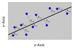
Figure 2. Geometric representation of the error-minimization model used by major axis regression analysis. In the actual calculations the sum of the squares of these distances is what is being minimized.
The line, passing through the bivariate centroid (¯X,¯Y), whose slope minimizes the sum of squares of these perpendicular deviation lines across the entire dataset represents, not only an intuitively reasonable trendline, but arguably the trendline we instinctively try to estimate through qualitative—or ‘eyeball’—inspection.
Calculations involved in estimating the major axis slope of a bivariate dataset are more complicated than those for the reduced major axis, but the necessary equations can be programmed into Excel easily. The equations given below are for reference only. They are implemented for the example trilobite data from last time in the Regressions II worksheet that can be downloaded here (please note the new information is situated as a new sheet in addition to the previous data in another sheet).
In order to better understand the calculation we need to deconstruct it into its parts. The first quantities needed are the variances of the two variables. These are most often calculated using an equation that is algebraically equivalent to equation 2.1, but more efficient computationally.
(2.4) s2=(∑x2i−((∑xi)2n))(n−1)
Next we need a single measure of the proportion of variance the two variables have in common, which is termed the covariance. Think of the variance being a one-dimensional measure of the distribution of observations about the mean (e.g., Fig. 1). The covariance is a two-dimensional measure of the spread of two variables around their joint mean (Fig. 3).
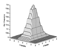
Figure 3. Joint probability distribution of two variables; (mean = 0.0, std. deviation = 1.0) and (mean = 0.0, std. deviation 0.5).
This is calculated by computing the sums of products for all paired variables.
(2.5) sx,y=(∑xiyi−(((∑xi)(∑yi))n))(n−1)
Once these values have been found an intermediate quantity must be calculated as follows.
(2.6) λi=0.5(s2x+s2y+√(s2x+s2y)2−4(s2xs2y−s2xy))
Calculation of the major axis slope is then a given by a simple equation.
(2.7) b=sx,y(λi−s2y)
Once the major axis slope value is in hand, the y-intercept of a line with this slope passing through the bivariate centroid is calculated in the manner described in the previous essay. Once again, these are somewhat involved formulae, but a worksheet is available to (1) illustrate the calculations and (2) enable you to simply copy your data into the example table, in which case the worksheet will calculate the major axis slope and intercept for you.
How does this method perform on our example trilobite data? Figure 4 summarizes the results obtained for four different regression analyses.
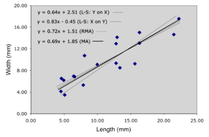
Figure 4. Alternative linear regression models for the trilobite glabellar length and width data used in to demonstrate reduced major axis regression.
The y on x and x on y least-squares regressions form an envelope within which the RMA and major axis (MA) models are contained. In data more symmetrically distributed about the linear trend, the RMA model usually bisects this envelope. The MA model exhibits a slightly lower slope than the RMA model because it is being ‘pulled’ in that direction by the greater variance associated with the length axis.
Which model is right? They all are. Each model minimizes a different aspect of variability about the linear trend. The answer to the more important question ‘Which is appropriate for my data?’ depends, as always, on the goal of the analysis. If your goal is to estimate the magnitude of one variable based on the value of another (e.g., body weight based on body length) least-squares regression offers the best option because it minimizes the estimation error. Alternatively, if you’re trying to quantify the pattern of linear covariation between gross dimensions measured in the same types of variables (e.g., linear distances between reference points), major axis regression would be the preferred choice because it (1) minimizes the joint deviations from the assumption of linearity in an intuitively reasonable manner and (2) takes differences in the scaling and magnitude between the variables into consideration. As for reduced major axis regression, I’d reserve this for situations in which you need to quantify the pattern of linear covariation between variables of intrinsically different types. Of course, these rules of thumb can be elaborated to cover a variety of situations. For example, what method would be most appropriate for estimating the magnitude of one variable based on the value of another when the two variables are of intrinsically different types? The following decision tree should help you make decisions regarding use of these models in your own work.
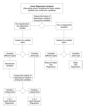
Figure 5. Decision tree
As I alluded to above, discussions of major axis regression are even rarer in statistical textbooks than discussions of reduced major axis regression. This is because the mathematics associated with major axis regression are necessarily bound up with the subject of eigenvalues—that ‘intermediate quantity’ we calculated in equation 2.6. This is one of the more complex concepts in linear algebra and one usually introduced in the context of matrix algebra. Sokal and Rohlf (1995) present the most complete discussion of the major axis approach in the context of regression of which I am aware. Davis (2002) mentions it under the name principal axis regression in his section on regression analysis, but refers the reader to his discussion of eigenvalues for computational details. Neither Swan and Sandilands (1995) nor Zar (1999) make any mention of major axis regression.
Reader's Comments:
Since this is column is intended to encourage discussion of quantitative data analysis topics, I’ll try to include a discussion/response to at least some of the comments and questions received from readers. Two comments stood out from your responses to the first essay. The first, from Andy L. A. Johnson of the University of Derby takes me to task for a mistake.
"One small correction for you to perhaps mention in your next piece: the critical 'slope' value which determines whether change in one variable is greater than that in the other is unity not 0.5 (see p. 30)"
Andy is correct. The sentence should read:
"Slope values of less than 1.0 (< 1.0) mean that a unit change in the x variable engenders a less than unit change in the variable. Slope values greater than 1.0 (> 1.0) represent mean that a unit change in the x variable engenders a greater than unit change in the yvariable.' and has been corrected in the on-line version of the essay."
This has been corrected in the on-line version of the Regression I essay. The error was typographical, but nevertheless my responsibility. The slope 1.0 has a special significance in studies of allometry (the study of the biological consequences of size change) where it corresponds to the limiting condition of perfect geometric scaling and is used to mark the interface between size/shape-change models that denote localized size changes that take place at a greater rate than overall size change (= positive allometry, β>1.0) from those models that denote localized size changes that take place at a lesser rate than overall size change (= negative allometry, β<1.0). In terms of ontogenetic allometry these models also have implications for morphogenic processes associated with the evolution of developmental programmes. We’ll be returning to these topics in future essays.
Claire Pannell of The University of Glasgow also wrote in with a warning about MS-Excel
"I would like to add a cautionary note on the use of Excel for statistics as I believe that Excel is at best unreliable and at worst incorrect in many of its formulae calculations. Excel is a good spreadsheet tool but not a statistical package and its algorithms are often unstable. There have been many criticisms about Excel voiced by many statisticians, which have never been resolved by Microsoft."
Claire is also correct. Excel is not an adequate substitute for a generalized statistical software package, though, as we have seen, these are by no means complete in terms of their respective approaches to, say, regression models. Excel’s problems appear to arise from some unfortunate choices in terms of the algorithms used to calculate various statistics. The problems are reasonably well known (e.g., statisticians delight in pointing them out), also exist in some dedicated statistical software packages (e.g., few packages implement Gurland and Tripathi’s 1971 correction factor for unbiased estimation of the standard deviation), and tend only to become noticeable when the magnitude of the numbers one is analysing becomes very large. Like all software, Excel is a tool and, like all tools, there are jobs for which it is suitable and jobs for which it is not. My preference for using Excel as a basis for exploring the methods discussed stems not from any inherent love of Excel as a computation platform (I much prefer Mathematica), but rather from the practical expectation that few will run out and purchase dedicated computational/statistical software just to follow this column. Interestingly, Excel’s well-known deficiencies have opened up the market for many third-party suppliers of statistical plug-ins, macros, virtual basic routines etc. designed to extend and correct this programme’s capabilities. Many of these are inexpensive ways to get high-quality stats capability on your computer. Sadly though, none includes the regression methods we have been discussing. Regardless, Excel’s errors need to be watched out for, so Claire’s advice is timely as well as correct. For those interested in learning more about what Excel can—and cannot—be expected to do, here are a few urls that will provide entry into this literature.
Helsel, D. R. 2002. Is Microsoft Excel an adequate statistics package?. http://www.practicalstats.com/Pages/excelstats.html
Goldwater, E. 1999. Using Excel for statistical data analysis. http://www-unix.oit.umass.edu/~evagold/excel.html
Pottel, H. 2002. Statistical flaws in Excel. http://www.mis.coventry.ac.uk/~nhunt/pottel.pdf
Excellent comments. Thanks to both Andy and Claire, and keep those e-mails coming.
Further Reading
Davis, J. C. 2002. Statistics and data analysis in geology (third edition). John Wiley and Sons, New York. 638 pp.
Gurland, J. and Tripathi, R. C. 1971. A simple approximation for unbiased estimation of the standard deviation. American Statistician 25: 30–32.
Jolicouer, P. 1975. Linear regressions in fishery research: Some comments. Journal of the Canadian Fisheries Research Board 32: 1491-1494.
Sokal, R. R. and Rohlf, F. J. 1995. Biometry: the principles and practice of statistics in biological research (third edition). W. H. Freeman, New York. 887 pp.
Swan, A. R. H. and Sandilands, M. 1995. Introduction to geological data analysis. Blackwell Science, Oxford. 446 pp.
Zar, J. H. 1999. Biostatistical analysis, Fourth Edition. Prentice Hall, Upper Saddle River, New Jersey. 663 pp.
Footnotes
1For a sample this average is calculated by dividing the degrees of freedom (n-1) into the sum of the squared deviations rather the sample size because the uncorrected average almost always underestimates the true population variance. See Gurland and Tripathi (1971) for discussion and an additional correction factor.
